Naive Bayes Classifer - Ziyue(Hadley) Hou

Definition

Naive Bayes classifiers are based on naive bayes classifier algorithms. Let’s say we have m input values $x_{ij}$

Assume all these input variables/features are conditionally independent given Y and equally contributed to the outcome.
In reality it is not quite possible that all features are conditionally independent

Simply chose the class label that is the most likely given the data, predict Y using $x_{ij}$

Bayes’ Theorem

Bayes’ Theorem gives the probability of an event occurring given the probability of another event that has already occurred.

$x_{ij}$

where y is class variable and $x_{ij}$ is a feature vector where $x_{ij}$

basically, we are trying to find probability of event y, given event x, event x is also termed as evidence.
p(x) is prior probability of x and p(y) is prior probability of y.
$p( \overrightarrow{x} |y)$ is a posteriori probability of y.

Since given assumption that all features are independent, then

$x_{ij}$

As the denomitor remains constant for a given input, we can obtain equations like follows:

$x_{ij}$

To maximize the probability of event y given the probability of event x is the same as to choose/calculate parameter y which result maximal probability using MAP:

$x_{ij}$

Compare between MLE and MAP

the key part difference is that prior distribution of unknown parameter is known or not, or is uniform or not.

Details can be found here:

wikipedia

MAP

MAP & MLE

Example

Outlook	Temperature	Humidity	Windy	Play Golf
Rainy	Hot	High	False	No
Rainy	Hot	High	True	No
Overcast	Hot	High	False	Yes
Sunny	Mild	High	False	Yes
Sunny	Cool	Normal	False	Yes
Sunny	Cool	Normal	True	No
Overcast	Cool	Normal	True	Yes
Rainy	Mild	High	False	No
Rainy	Cool	Normal	False	Yes
Sunny	Mild	Normal	False	Yes
Rainy	Mild	Normal	True	Yes
Overcast	Mild	High	True	Yes
Overcast	Hot	Normal	False	Yes
Sunny	Mild	High	True	No

Task: estimate whether or not to play golf when it’s {Rainy, Hot, High, False}

Solution:

$x_{ij}$

Given specific observations mentioned in the task:

$x_{ij}$

Now after normalization or logarithmic calculation, we compare both probabilities for playing gold and not playing gold, and the prediction would be the one with higher probability:

$x_{ij}$

Implementation continuous data model from scratch

Import module

import numpy as np
from sklearn.model_selection import train_test_split
from sklearn import datasets
import matplotlib.pyplot as plt

Input datasets

X, y = datasets.make_classification(n_samples=1000, n_features=10, n_classes=2, random_state=123)
X_train, X_test, y_train, y_test = train_test_split(X,y,test_size=0.2,random_state=123)
print(X.shape)
print(y.shape)
print(X[0:5])
print(y[0:10])

(1000, 10)
(1000,)
[[ 0.24063119 -0.07970884 -0.05313268  0.09263489 -0.13935777  1.20319285
  -0.15590018 -0.09709308  0.06994683  0.11660277]
 [ 0.75425016 -0.937854    0.21947276 -1.28066902  1.55618457 -0.65538962
   0.77023157  0.19311463 -2.27886416  0.65102942]
 [ 0.9584009  -1.31841143  1.15350536 -0.96816469  1.88667929  0.53473693
   0.46015911  0.0423321   0.79249125  0.24144309]
 [ 0.64384845  0.35082051 -0.10869679  0.71060146 -0.85406842  0.33485545
   0.60778386  0.94834854  1.29778445  2.16583174]
 [ 1.03268464 -1.26482413  0.18067775  0.35989813 -0.26303363 -0.33760592
   0.52075594 -1.4403634   1.25766489  0.14630826]]
[0 0 1 1 1 0 0 0 1 0]

create naive bayes model

class NaiveBayes:
    def fit(self, X, y):
        self._samples, self._features = X.shape
        self._classes = np.unique(y)
        self._labels = len(self._classes)

        # initialize mean, var, and prior for each feature
        self._mean = np.zeros((self._labels, self._features), dtype=np.float64)
        self._var = np.zeros((self._labels, self._features), dtype=np.float64)
        self._priors = np.zeros(self._labels, dtype=np.float64)

        # calculate mean, var and prior for each feature given y
        for i,label in enumerate(self._classes):
            temp = X[y==label]
            self._mean[i,:] = temp.mean(axis=0)
            self._var[i,:] = temp.var(axis=0)
            self._priors[i] = temp.shape[0]/float(self._samples)
    
    # calculate posterior for each class given observed dataset x
    def _train(self, x):
        posteriors = []

        for i, label in enumerate(self._classes):
            prior = np.log(self._priors[i])
            posterior = prior + np.sum(np.log(self._pdf(i,x)))
            posteriors.append(posterior)
        
        # compare and return highest posterior probability
        return self._classes[np.argmax(posteriors)]


    # calculate pdf for each row of observed dataset x
    def _pdf(self, index, x):
        mean = self._mean[index]
        var = self._var[index]
        numerator = np.exp(-(x-mean)**2 / (2*var))
        denominator = np.sqrt(2*np.pi*var)
        return numerator/denominator  

    # predict test data
    def predict(self, X):
        y_pred = [self._train(x) for x in X]
        return np.array(y_pred)
    
    # calculate accuracy
    def accuracy(self, y_test, y_pred):
        accuracy = np.sum(y_test == y_pred) / len(y_test)
        return accuracy

nb = NaiveBayes()
nb.fit(X_train, y_train)
print(nb._classes)
print(nb._samples)
print(nb._features)
print(nb._labels)
print(nb._mean.shape)
print(nb._var)
print(nb._priors.shape)
print(nb._pdf(0,X[0]).shape)
y_pred = nb.predict(X_test)
print(nb.accuracy(y_test,y_pred))

[0 1]
800
10
2
(2, 10)
[[0.98269025 0.95576451 0.36205835 0.44312622 1.29896635 0.86864312
  1.03288266 0.89110435 0.33131845 0.95275246]
 [1.03305993 0.95375061 0.48209481 0.59179712 1.7236553  0.92576642
  0.96969459 1.10314154 0.50775021 1.14787765]]
(2,)
(10,)
0.965

nb = NaiveBayes()
nb.fit(X_train, y_train)
y_pred = nb.predict(X_test)
accuracy = nb.accuracy(y_test,y_pred)

print("Naive Bayes classification accuracy", accuracy)

Naive Bayes classification accuracy 0.965

Implementation using sklearn

import modules

import numpy as np
import pandas as pd
import matplotlib.pyplot as plt
import seaborn as sns
from sklearn.model_selection import train_test_split
from sklearn import datasets

import datasets

X, y = datasets.make_classification(n_samples=1000, n_features=10, n_classes=2, random_state=123)
X_train, X_test, y_train, y_test = train_test_split(X, y, test_size=0.2, random_state=123)

Model Training

from sklearn.naive_bayes import GaussianNB

nb = GaussianNB()
nb.fit(X_train, y_train)

GaussianNB()

Predict the results

y_pred = nb.predict(X_test)
y_pred.shape

(200,)

from sklearn.metrics import accuracy_score

print('Model accuracy score: {0:0.4f}'. format(accuracy_score(y_test, y_pred)))

Model accuracy score: 0.9650

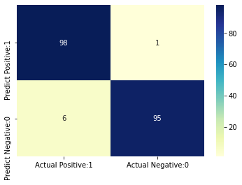
Confusion Matrix

from sklearn.metrics import confusion_matrix

confusion_matrix = confusion_matrix(y_test, y_pred)
print('Confusion matrix\n\n', confusion_matrix)

Confusion matrix

 [[98  1]
 [ 6 95]]

Visualize confusion matrix

cm_matrix = pd.DataFrame(data=confusion_matrix, columns=['Actual Positive:1', 'Actual Negative:0'], 
                                 index=['Predict Positive:1', 'Predict Negative:0'])

sns.heatmap(cm_matrix, annot=True, fmt='d', cmap='YlGnBu')

<AxesSubplot:>

svg